Python Tutorial — Colab Notebook Answer Key

Last Updated: April 23, 2026 Download notebook (.ipynb)

Author: Answer Key

Our research this semester will focus on determining the efficiency of solar cells and how this changes as we stress the cells. To be able to do this research, you will need to be able to do some simple analysis, and we have chosen python using Google Colab as the platform. Python is now one of the most common languages used in science and Colab is easy to use as you don't need to install anything directly on your computer. It is also very easy to share documents with your team members.

In this assignment, we will learn all the basic data analysis tools we will be using this semester and explore a programming language called Python. We will be using sample data from solar cells. By the end, you will be able to determine the paramerters from the raw data you will take throughout the semester!

1 Introduction to using Python and Google Colaboratory

To analyze our data for our semester-long solar cell project, we will be using code in the Python programming language. Maybe you have been writing Python all your life, or maybe you are just hearing about it for the first time. Either way is just fine! We do not assume you have any prior knowledge. If you do, just bear with us, as we get everyone up to speed.

We will be learning Python the same way lots of scientists first learn a new programming language: Not with a formal course, but just by looking at examples of the code in action and then playing around with it and modifying it to see what they can change.

To use a Python program, you also have to have a place to write and run this code. In this course, we will use a tool called Google Colaboratory, or just "Google Colab" for short. That is the page you are on right now, in fact. Colab lets you combine written words like this ("rich text") and Python code you can actually run ("executable code"), which you will see below.

2 Overview of the Tutorial

This Python/Colab tutorial will walk you through examples of coding that will be helpful during your data analysis this semester. There are also 13 problems throughout the tutorial that will let you practice these skills. The problems can be found in the following sections of the tutorial:

Problem 1: Formatting text in Colab using "markdown" cells
Problem 2: Introduction to Python coding
Problem 3: Writing readable code and commenting
Problem 4: Data Structures
Problem 5: Using functions from Python libraries 1
Problem 6: Using functions from Python libraries 2
Problem 7: J-V Calculations
Problem 8: Power Conversion Efficiency 1
Problem 9: Power Conversion Efficiency 2
Problem 10: External Quantum Efficiency 1
Problem 11: External Quantum Efficiency 2
Problem 12: AI disclosure
Problem 13: AI practice (required)

This is an individual assignment. This means you can ask your teammates and TA for help, but the work must be completed on your own. See Canvas for the due date. If you need help after your lab section, please attend any of the TA office hours listed on Canvas.

Let's get started!

3 Formatting text in Colab: A guide to "markdown"

Before we even get to the python, let's start by learning how to enter text and format it in Google Colab. We will need this to be able to write about our research and our results along the way. We'll be using something called "markdown."

3.1 What is markdown?

Google Colab notebooks are broken up into sections called "cells." Cells are either text cells, like this one, or code cells, where you will write and run python code.

Choose a text cell somewhere in this notebook and double click on it. You will pull up the markdown that was used to make the text appear the way it does.

3.2 Using Markdown

Here are a few common text formatting things you might want to do with markdown. You can find many more things that markdown can do by searching online for things like "markdown reference" or "markdown cheat sheet." Here is one, for example.

To make a bulleted list (like this one!) type a dash (-) at the beginning of the line, with a space after it.
- Lists can be nested (like this!) using two spaces in front of the dash for each level of nesting.
  - See?
To make text bold surround it with **two asterisks**.
To make text italic surround it with *single asterisks*.
Text formatted like this is called "monospace". It's traditionally used for examples of code in the middle of regular text. To make your text look like this, surround it by the "backtick" symbol (on the same key as the tilde (~) symbol): `

Markdown also has a built-in way to display professional looking mathematical equations, using another text language called "LaTex" (usually pronounced "lay-tech" or "lah-tech").

To type an equation, surround it with dollar signs. Between the dollar signs, you can use LaTex notation to make the equations come out looking proper. For example, typing " $E = mc^2$ " renders as $E = mc^2$.

A few common bits of LaTex notation you may want to know:

To get a greek character like $\lambda$, type its name with a backslash before it ( $\lambda$ )
Underscores create subscripts like in $\mu_k$ ( $\mu_k\$ )
The up caret "^" create superscripts like in $\pi r^2$ ( $ pi r^2$ )
To express a square root like $\sqrt{2}$, use $\sqrt{2}

This should give you more than you need for our course, but if you want more detailed markdown instructions, you can check out GitHub's documentation. GitHub is a website that is widely used by anyone who needs to write, share, and collaborate on code, and they use a very similar (though not identical) version of markdown.

3.3 Problem 1

Now: Your turn to try formatting text. Use the guide above and/or the editing toolbar at the top of the window, and talk with your classmates and TAs if you need help!

To enter some text, create a text cell below. Hover your mouse below this cell and click on "+ Text" when it appears.
Edit the text cell you created by double clicking on the new cell you created.
Write a sentence with one word in bold and one in italics.
Write a phrase using monospace.
Format your favorite equation using LaTex (choose something with at least one feature that couldn't easily be expressed in plain text, like a Greek character, an exponent, etc).
Create a bullet point list of any questions or concerns you have so far.

3.4 `Problem 1 Solution`

Bold and italics (4): Text has been entered.

Monospace (5): This is a monospace phrase.

Favorite Equation (6): $L_{Edd} = \frac{4\pi GMm_{p}c}{\sigma_{T}}$

Bullet list (7):

List of concerns item 1
List of concerns item 2

4 Introduction to Python coding

Alright, let's learn to work with Python code, so we can use it to analyze data from our solar cells.

Python is a powerful, high-level programming language designed to be easy to read (compared to some other languages). It is currently ranked as one of the most popular programming languages globally.

Don't forget, you don't need to learn to code from scratch. We just want you to be able to take Python code that you see and adapt it or customize it to your own needs.

Below is a code cell with a short Python script that computes a value, stores it in a variable, and prints the result:

seconds_in_an_hour = 60 * 60
print(seconds_in_an_hour)

To execute the code in the above cell, select it with a click and then either press the play button to the left of the code, or use the keyboard shortcut "Command/Ctrl+Enter" (to use the keyboard shortcut, the code cell needs to be active - you can do this by clicking on the cell). To edit the code, just click the cell once and start editing.

This code defines a variable which is equal to 60 times 60. Then, it prints the value of that variable.

After being executed, variables that you define in one cell can also be used later in other cells:

seconds_in_a_day = 24 * seconds_in_an_hour
print(seconds_in_a_day)

When coding, variable names are case-sensitive. For example, if I wrote:

seconds_in_a_day = 24 * seconds_in_an_hour
print(Seconds_In_A_Day)

---------------------------------------------------------------------------
NameError                                 Traceback (most recent call last)
/tmp/ipython-input-734979218.py in <cell line: 0>()
      1 seconds_in_a_day = 24 * seconds_in_an_hour
----> 2 print(Seconds_In_A_Day)

NameError: name 'Seconds_In_A_Day' is not defined

I get an "error" that says NameError: name "Seconds_In_A_day" is not defined", which is true because only "seconds_in_a_day" (lower case!) exists!

4.1 Problem 2

Create a new code cell by hovering your mouse below this cell and clicking + Code.
Copy and paste the code from the previous code cell that produced an error into your new code cell. Edit the code to correct this error.
On a new line in the same code cell, write 'print("The number of seconds in a day is ", seconds_in_a_day)' and run the cell. Can you figure out how this new bit of code is working?
On a new line in the same code cell, write some code that uses the variable 'seconds_in_a_day' to calculate the number of seconds in a week. Name the new variable 'seconds_in_a_week'.
By adapting the example code, write another line of code that prints a sentence telling us the number of seconds in a week. ___

4.2 `Problem 2 Solution`

seconds_in_a_day = 24 * seconds_in_an_hour
print(seconds_in_a_day)             #correct the formatting of the error

seconds_in_a_week = 7 * seconds_in_a_day  #define new variable
print(seconds_in_a_week)                  #print new variable

86400
604800

5 Writing readable code

Sometimes, you want to include comments about your code along the way, line by line. This is called commenting your code.

In Python, you can do this by using a hashtag. Everything after the hashtag is treated as text, rather than code, so the computer will not try to run it. Note, Markdown does not work within a code comment like this.

To see what code commenting looks like, read through the code below, and see if you can figure out how it works by reading the comments (if it doesn't completely make sense to you yet, that is okay).

primes = [2, 3, 5, 7, 11] # create a list of numbers
print("The first prime number is", primes[0]) # print the first item in the list of primes.

The first prime number is 2

5.1 Problem 3

Create a new code cell by hovering your mouse below this cell and clicking + Code.
Copy and paste your code from Problem 2, but this time, add some comments to explain each step.

By the way, more than one scientist has been embarrassed over the years because of something they wrote as a comment in their code that they did not expect anyone else to see. Always assume your comments will eventually be public! ___

# I already commented my code above, so I just added some more. Use your judgement!

seconds_in_a_week = 7 * seconds_in_a_day  # (2) define and calculate new
                                          # variable called seconds_in_a_week

print(seconds_in_a_week)                  # print seconds_in_a_week variable

6 Data Structures

6.1 Lists and Arrays

As you just saw in the previous example, one thing you can do in Python is create "lists." In fact, lists are one of the central features of Python.

Think of a list like a shopping list or a to-do list. You can store anything in a list, and the order you add things matters! For instance, you might have a list that stores the electrical currents measured in a solar cell at different voltage levels.

In Python, lists are written with square brackets, with the items separated by commas. The items in a list can be numbers, text, or even other things.

Let's look at an example using text (called "strings"). Notice that strings are always placed in quotation marks.

quarks = ["up", "down",  "charm", "strange", "top", "bottom"]   # List of types of quarks
print(quarks) # Print the list to make sure it looks right

# Does writing this code make us "string" theorists?

['up', 'down', 'charm', 'strange', 'top', 'bottom']

Another data structure is an array. An array compactly represents a group of basic values: characters, integers, floating-point numbers. Arrays behave very much like lists, except that the type of objects stored in them is constrained.

Let's look at an example array of random integers.

import numpy as np      # In order to use an array, you need to import the Numpy library
                        # We will discuss libraries later

my_list = [5, 8, 1, 6, 3, 14, 6, 20, 13, 25, 10]  # Create the variable "my_list" with some random data
my_array = np.array(my_list) # Converts the Python list into a NumPy array using the np.array() function.

print(my_array)

[ 5  8  1  6  3 14  6 20 13 25 10]

If you want an individual element of a list or an array, you refer to it with its "index number." You can do the same thing if you want a subset of the list. This will be a very important skill for us! That is how we will access the particular datapoints we are interested in.

For example:


print(quarks[0]) # Prints the first element of the list
print(quarks[3]) # Prints the fourth element of the list (not a typo! see below)

up
strange

Notice: The first item in a list is called "item 0" not "item 1". So to get the first quark on the list, we use quarks[0], to get the second quark we use quarks[1], etc.

Now, suppose you want not just a single element, but a subset of a list ("slicing" the list). Here's how we do that:

print(my_array[3:6]) # Print the fourth, fifth, and sixth elements of the integer array

[ 6  3 14]

6.2 Problem 4

Create a new code cell below.
Make a list of the first ten integers: [1, 2, 3, 4, 5, 6, 7, 8, 9, 10] and give it a variable name.
Using indexing to print the item at the 5th index. Explain in a comment what output to expect and why.
Use slicing to create a new list with only the numbers 7, 8, and 9. ___

6.3 `Problem 4 Solution`

integer_list = [1, 2, 3, 4, 5, 6, 7, 8, 9, 10]    # (2) Variable name will differ

print(integer_list[5])      # (3) Printing 5th index, and additional note to why
                            # they expect the number they got in comment

slice_index = integer_list[6:9]     # (4) Define sliced index - they may or may
print(slice_index)                  # not print the variables, but they were
                                    # only asked to create the list, not print it

6
[7, 8, 9]

Lists are just one way of representing collections of datapoints in Python. In this course, we will use something similar, but more advanced, called a dataframe.

6.4 Working With Dataframes

We practiced storing and accessing data in lists because those are the most basic objects in Python. But for our research, we will need a more complex datatype called a "dataframe" to store and manipulate our solar cell data. Fortunately, many of the basic ideas you just learned about lists will still apply.

Dataframes are part of the pandas library (similar to how arrays are part of the numpy library), so we need to import the library with the following code:

import pandas as pd

Note: python libraries often had goofy names that do not tell you about what they actually do.

Dataframes are useful in part because they can easily store data in a "table", with multiple columns. They also make it easy to import raw data from a .csv file.

Let's try this out. This time, we will practice with a dataframe containing some "test" solar cell data.

You should find a .csv file with the "test" solar cell I-V data on this week's page in Canvas - the file is called tutorial_iv_current_voltage.csv'. Download that .csv file onto your computer and upload it into this Google Colab notebook. To upload into this notebook click on the file icon on the left side of your screen. Then click on the "upload to session storage" icon.

Find where you downloaded the .csv file onto your computer and click open.

You should now be able to run the code cell below.

import pandas as pd                 #Import pandas library

df = pd.read_csv('tutorial_iv_current_voltage.csv')    # We will read in the data
                                    # from the csv and store it as a dataframe
                                    # called "df". When you are working with
                                    # your real data you will need to change
                                    # the name of the .csv file in your code to
                                    # match the  name of the .csv that has
                                    # your data.

display(df)       # Display the dataframe, df. See how it's basically a data table

	Voltage (V)	Forward_mean (mA)	Forward_std (mA)	Forward_n	Reverse_mean (mA)	Reverse_std (mA)	Reverse_n
0	-0.20	-1.33318	0.001686	10	-1.26615	0.001865	10
1	-0.18	-1.32479	0.000489	10	-1.26168	0.002892	10
2	-0.16	-1.31941	0.001788	10	-1.25965	0.003597	10
3	-0.14	-1.31529	0.001358	10	-1.25644	0.001943	10
4	-0.12	-1.31018	0.002892	10	-1.25336	0.002700	10
...	...	...	...	...	...	...	...
81	1.42	2.20997	0.001943	10	2.30676	0.059868	10
82	1.44	2.27217	0.002254	10	2.45429	0.004455	10
83	1.46	2.33821	0.001512	10	2.55304	0.001525	10
84	1.48	2.41264	0.004178	10	2.64690	0.002701	10
85	1.50	2.48875	0.004511	10	2.73594	0.002980	10

86 rows × 7 columns

Selecting data from a dataframe

One thing we will be doing over and over again in this project will be taking some data in a dataframe and then choosing only a specific subset of that data to look at.

There are a few different ways you could do this. One simple way is that you can select just a single column of the data by referencing its title. For example, if you wanted to display only the second column, titled "Forward_mean (mA)", you can do the following:

display(df['Forward_mean (mA)'])  # Display only the Forward Scan current column

	Forward_mean (mA)
0	-1.33318
1	-1.32479
2	-1.31941
3	-1.31529
4	-1.31018
...	...
81	2.20997
82	2.27217
83	2.33821
84	2.41264
85	2.48875

86 rows × 1 columns

dtype: float64

Keep in mind how you called the Forward mean column. We will come back to handling data in dataframes, but first let's go over a few other Python basics.

7 Using functions from Python libraries

In Python, you can think of a function as a reusable block of code that performs a specific task. This concept is similar to the mathematical definition of a function, but it's more flexible. In Python, a function can handle various inputs and produce outputs, just like a mathematical function, but it can also perform actions beyond simple calculations, such as interacting with files or displaying information.

7.1 Built-In Functions

We have already seen some functions that are built-in to Python, like print(). They perform convenient actions all in one step. We will use them to manipulate our data.

A few other common built-in functions:

len()
sum()
max()
min()
sorted()

Each function has certain rules involved with using it. Here is a link to a full list of how to use the built-in functions: https://docs.python.org/3/library/functions.html. For example, when you look up the function len() is says:

len(s) — Returns the length (the number of items) of an object. The argument may be a sequence (such as a string, bytes, tuple, list, or range) or a collection (such as a dictionary, set, or frozen set).

So, this function tells you the length of whatever you put inside the parentheses (the "argument").

Look at the code cells below to see some other functions at work. Try to guess what the output will be. Then, run each piece of code and see if your prediction was correct!

my_list = [5, 8, 1, 6, 3, 14, 6, 20, 13, 25, 10]
print(my_list)

[5, 8, 1, 6, 3, 14, 6, 20, 13, 25, 10]

max(my_list)

sorted(my_list)

[1, 3, 5, 6, 6, 8, 10, 13, 14, 20, 25]

7.2 Problem 5

Create a new code cell below.
Use one of the functions listed above to find the sum of all the elements in my_list.
Use one of the functions listed above to find the sum of just the FIRST THREE elements of my_list. ___

7.3 `Problem 5 Solution`

sum(my_list)        # (2) find sum of my_list

sum(my_list[0:3])   # (3) find sum of 5+8+1

7.4 Python libraries

These built-in functions are limited. Luckily, since Python is open-source, you can use functions that other people have written. A collection of functions someone else has written for use in Python is called a library.

To use the functions in one of these libraries in Google Colab, you will need to "import" the libraries in every new colab notebook before you can use their functions.

Two famous python libraries you will use often are called numpy (which you have already imported above!) and pyplot, which is a library within within matplotlib.

from matplotlib import pyplot as plt   # Here we import pyplot from matplotlib
                                       # and call it plt

Execute the code in the above. These two libraries are now imported and the functions within them are now available to you in this notebook just like the built in functions were.

This semester we will be using numpy, matplotlib, and pandas a lot, so feel free to copy and paste whenever you need access to these libraries of functions.

7.5 Basic Plotting

Let's put these new functions to use. We will eventually want to plot our data, so to practice, let's use the dataframe we imported and use plot() to make a graph of it.

Notice how we use these functions: since they come from a library, we have to tell Python which library to get them from. Instead of just writing "plot" we write (plt.plot), which means "the plot function found within the pyplot library that we nicknamed "plt".)

Try executing the code below. Note: If you see an error that says "NameError: name 'plt' is not defined" then it is telling you that the library has not actually been imported correctly. Make sure you have executed the code cell above that imports the two libraries.

Now let's plot the Forward Scan for pixel 1 against the Voltage.


plt.plot(df['Voltage (V)'] ,df['Forward_mean (mA)'],'k.', label = 'Forward Scan')  # Plot the Forward Scan data for Pixel 1.
                                                    # The function plot() inside the library pyplot
                                                    # (which we called plt) will plot the Forward Scan vs
                                                    # the Voltage from the dataframe using a
                                                    # small point (.) in the color black ("k")

plt.title("Solar Cell I-V Curve (Pixel 1)")         # We can also use the function title() to add a
                                                    # title to our plot. Notice the quotation marks
                                                    # around the text
plt.ylabel("Current (mA)")       # Creates axis label for y-axis. Always include units if you have them
plt.xlabel("Voltage (V)")        # Creates axis label for x-axis
plt.legend()                     # Prints label for data points
plt.show()                       # Last, we use the fuction show() to display
                                 # the plot when we execute the code. Notice
                                 # this has to come AFTER the code where we add
                                 # the plot title.

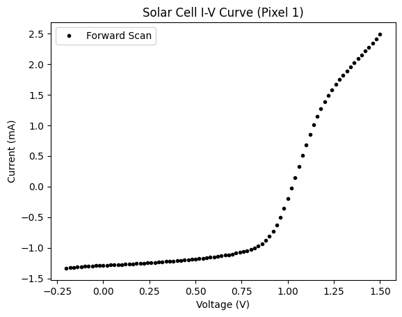
Nice! We can clearly see the current through the solar cell rises sharply as we increase the voltage. The general shape of this plot should look like what you saw in lecture and in the papers. It may look upside down compared with what you have seen as there is no standard for which way to plot the vertical axis.

7.6 Problem 6

Create a new code cell below.
Copy the plotting code for the Forward Scan from the code cell above into the new code cell you just created.
For our measurements this semester, we will be using the Reverse Scan values. Edit the code (and the comments!) so that it plots the Reverse Scan column instead of the Forward Scan column.
Edit the code by replacing the point '.' with an asterisks '*', and run the code. In a comment, describe how this affected the plot.
Replace 'k' with 'r' and run the code. See if you can guess what the "r" meant.
Based on what you've seen so far, figure out how to change the code so that it plots the Reverse Scan with blue triangles. ___

7.7 `Problem 6 Solution`

# (2 and 3)Plot the Reverse Scan data for Pixel 1.
plt.plot(df['Voltage (V)'] ,df['Reverse_mean (mA)'],'b^', label = 'Reverse Scan')


plt.title("Solar Cell I-V Curve (Pixel 1)")         # We can also use the function title() to add a
                                                    # title to our plot. Notice the quotation marks
                                                    # around the text
plt.ylabel("Current (mA)")       # Creates axis label for y-axis. Always include units if you have them
plt.xlabel("Voltage (V)")        # Creates axis label for x-axis
plt.legend()                     # Prints label for data points
plt.show()                       # Last, we use the fuction show() to display
                                 # the plot when we execute the code. Notice
                                 # this has to come AFTER the code where we add
                                 # the plot title.

# (3) they should have a comment saying when they replace '.' with '*' it changes
# the data point from a dot to a star

# (4) they should have a comment saying they think it will change the plot points
# to red

# (5) The final plot that is printed should have blue triangles, which you can
# see below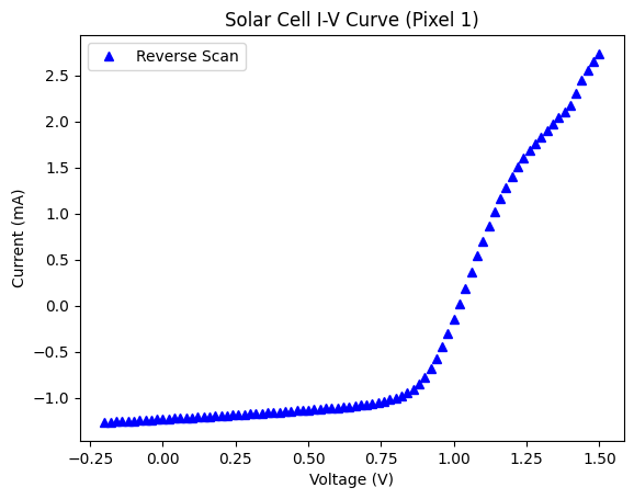

8 J-V Calculations

In addition to plotting, we can manipulate numerical columns in dataframes using mathematical functions. When you are doing analysis with your team's cell, you will need to convert from current to a current density in order to find some important values. The symbols for basic math function are - add: +, subtract: -, multiply: *, divide: /.

Current density, J, is the measure of the flow of electric charge per unit area. Example units of this would be $mA/cm^2$. The cell that was used to create this test data has a nominal active area of 0.14 $cm^2$ and the current is in $mA$, so to calculate the current density we need to divide the current by the active area of the cell.

jv_columns = {                                                     # Create a list to name, select and edit the columns you want from the I-V dataframe
    'Voltage (V)':df['Voltage (V)'],                                       # Want voltage and it can stay the same
    'Current Density (mA/cm^2)' : df['Reverse_mean (mA)']/0.14            # We want current density instead of current, we divide a current column from
              }                                                    # the previous data frame (mA) by the active area of the cell (cm$^{2}$)


jv_pix1 = pd.DataFrame(jv_columns)                                  # Once your list is made, create a new data frame for your J-V plot

display(jv_pix1)                                                    # Display your new J-V data frame

8.1 Problem 7

Create a new code cell below.
Create a plot showing Current Density versus Voltage.
Use the plt.ylim() function to switch the direction of your y-axis so the negative numbers are on top.
Update the Title, x- and y- axis labels. ___

8.2 `Problem 7 Solution`

# (2) Some reasonable thing to make the plot
plt.plot(jv_pix1['Voltage (V)'] ,jv_pix1['Current Density (mA/cm^2)'],'k.')

# (3) updated y-axis range
plt.ylim(15, -23)

# (4) udated title and axes labels
plt.title("Solar Cell J-V Curve (Pixel 1)")
plt.ylabel("Current Density (mA/cm$^2$)")
plt.xlabel("Voltage (V)")

plt.show()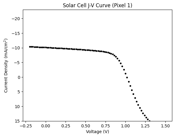

9 Power Conversion Efficiency

Now that we have both our I-V and J-V plots, what we really want to determine is the Power Conversion Efficiency, which is also called PCE or $\eta$. The PCE is a measurement of how well the cell converts light energy into electrical energy. It is calculated by dividing the output electrical power by the input light power and expressing the result as a percentage, and is calculated by this equation:

$PCE = \frac{V_{OC} * J_{SC} * FF}{P_{in}}$

That is a lot of varibles, so what do all of them mean and how do we determine them from our data?

Let's start with the open circuit voltage, or $V_{OC}$. On the J-V plot, you can find $V_{OC}$ where the current is zero ($J = 0$). So lets search the dataframe using the interp() function.

v_oc = np.interp(0,jv_pix1['Current Density (mA/cm^2)'], jv_pix1['Voltage (V)']) #inside the brackets (value we want to find, variable_1, variable_2)
                                              # so in our case, we want to find 0, for the forward scan current (variable 1)
                                              # and want it to tell us what the Voltage is for that current (variable 2)
print(v_oc)

1.0179186275093823

Go back and look at your J-V curve. Does the value that was found make sense?

Next, let's find the short circuit current, or $J_{SC}$. On the J-V plot, you can find $J_{SC}$ where the voltage is zero ($V = 0$). Because of the voltage steps in our measurement we do have a $V = 0$ value, we can search for the index of the row that corresponds to $V = 0$, using the index function on our J-V data frame.

jsc_index = jv_pix1.index[jv_pix1['Voltage (V)'] == 0]               # Using the index function we can find the row number

print(jsc_index)                                                 # Print to check that you indexing worked!

Index([10], dtype='int64')

Now that you know what row of your J-V data frame has a zero voltage value, let's assign the corresponding current density to a variable.

j_sc = jv_pix1.loc[jsc_index,'Current Density (mA/cm^2)'].values[0]              # Using loc we can use the index number for V = 0 and
                                                                       # find it's corresponding voltage and current density

print(j_sc)                                                            # Display row from J-V data frame

-10.113606557377048

Third, we need to find the Fill Factor, or FF. FF is a measurement that assesses the efficiency of a solar cell by comparing its actual power output to its maximum possible power output. It is calculated from the following equation:

$FF = \frac{J_{pmax} * V_{pmax}}{J_{SC} * V_{OC}}$

We have already found $J_{SC}$ and $V_{OC}$, so now we need to find $J_{pmax}$ and $V_{pmax}$.

First, create a voltage versus power plot, just so you know what it looks like, by plotting Voltage on the x-axis and Power (=Voltage * Current Density) on the y-axis.

plt.plot(jv_pix1['Voltage (V)'], jv_pix1['Voltage (V)']*jv_pix1['Current Density (mA/cm^2)']) # Creates new Voltage vs. Power plot

plt.ylim(15, -15)                                                            # Similar to J-V plot switch the limits for y-axis
                                                                            # so negative numbers are on top
plt.title("Solar Cell Power Curve (Pixel 1)")         # Title for plot

plt.ylabel("Power (mW/cm$^{2}$)")       # Creates axis label for y-axis. For the units remember
                                        # V * mA = mW and since its a current density we still have
                                        # the cm^2
plt.xlabel("Voltage (V)")        # Creates axis label for x-axis
plt.show()                       # Last, we use the fuction show() to display
                                 # the plot when we execute the code. Notice
                                 # this has to come AFTER the code where we add
                                 # the plot title.

Now, let's find the maximum power value and its corresponding voltage ($V_{pmax}$) and current density ($J_{pmax}$), using the numpy argmin() function, which returns the index of the smallest element of an array.

Wait! If we are looking for the maximum power value why are we looking for the smallest number? We will cover this more in a future photovoltaics lecture, but for now know the negative sign has to do with the direction of the voltage versus current.

power=jv_pix1['Voltage (V)']*jv_pix1['Current Density (mA/cm^2)']                         # Creating an array of power values

pmax_index = np.argmin(power)                                                # Use argmin to search the power array and find the max power index
                                                                             # which we will use to find the corresponding Voltage value

print(pmax_index)                                                            # This print statement shows us what the index number is for the max power

Now that we know the index number for the maximum power value, we can find the corresponding voltage and current density from our J-V data frame.

v_pmax = jv_pix1.loc[pmax_index,'Voltage (V)']                             # Using loc we can assign values from the row with V = 0
j_pmax = jv_pix1.loc[pmax_index,'Current Density (mA/cm^2)']                     # to variables

print(v_pmax)                                                          # A print check to see that your variable assignment worked
print(j_pmax)

0.8
-8.207786885245902

Using your $V_{pmax}$ value, check your voltage versus power plot to see if this make sense. If yes, you can use basic math functions (* and /) to calculate the fill factor, FF, which is defined as:

$FF = \frac{J_{pmax} * V_{pmax}}{J_{SC} * V_{OC}}$

9.1 Problem 8

Create a new code cell below.
Using basic math functions, define and calculate FF.
Use a print statement to show the value of FF. ___

9.2 `Problem 8 Solution`

# (2) create variable and do the calculation
ff = (j_pmax*v_pmax)/(j_sc*v_oc)

# (3) print variable value
print(ff)

0.637818250623082

Now that we have all of our variables we are ready to calculate the Power Conversion Efficiency! As a reminder PCE is defined by the following equation:

$PCE= \frac{V_{OC} * J_{SC} * FF}{P_{in}}$

The one variable we did not calculate is $P_{in}$, which is the power of the light from the solar simulator hitting the pixel (which is in units of Power/Area). This value (and other details) can be found in the Ossila Solar Simulator Calibration Certificate on the 'Other Resources' Canvas page. For simplicity, we will provide this value: $P_{in} = 99.8 mW/cm^{2}$. Make a note so you can use it for your analysis going forward!

9.3 Problem 9

Create a new code cell below.
Create a variable defining $P_{in}$ as the value given above.
Using the equation above, calculate the PCE (η).
Print the calculated PCE value.
Using the abs() function, convert the PCE to a percent value instead of a fractional value.
Create a print statement that says 'The PCE value is:' with the percent value. ___

9.4 `Problem 9 Solution`

# (2) define p_in

p_in = 99.8

# (3) define pce variable and calculate with basic math functions
pce = (v_oc*j_sc*ff)/p_in

# (4) print pce value
print(pce)

# (5) define and do absolute value and multiply by 100 to turn into percent
pce_percent = abs(pce)*100

# (6) print statement for precent pce value
print('The PCE value is: ',pce_percent,'%')

-0.06579388284766255
The PCE value is:  6.579388284766255 %

10 External Quantum Efficiency

Now that we have calculated our PCE value using our J-V data, we can turn our attention to our External Quantum Efficiency, or EQE, data. There will be two files that you will collect from each EQE measurement - a file with current data and a file with power data. To begin, let's define some constants that we will need for our calculations.

# Constants
h = 6.62607015e-34  # Planck's constant (Joule second)
c = 3.0e8  # Speed of light (meters per second)
e = 1.602176634e-19  # Elementary charge (Coulombs)
active_area_cm2 = 0.14  # Active area in cm^2
active_area_m2 = active_area_cm2 * 1e-4  # Convert cm^2 to m^2

Next, we need to read in our EQE data files and convert wavelength from nanometers to meters and calculate our EQE values.

# Read the data from the CSV files
power_data = pd.read_csv('tutorial_eqe_power.csv')
current_data = pd.read_csv('tutorial_eqe_current.csv')

# Convert units
power_W = power_data['Power_mean (uW)'] * 1e-6       # Convert uW to W
current_A = current_data['Current_mean (nA)'] * 1e-9  # Convert nA to A
wavelength_meters = current_data['Wavelength (nm)'] * 1e-9  # Convert nm to meters

# Calculate the EQE
eqe = (current_A / power_W) * (h * c / (e * wavelength_meters))

Now that you have your new variables - wavelength in meters and the EQE values, make a new dataframe to store your data.

10.1 Problem 10

Create a new code cell below.
Create a new dataframe to store the wavelength and EQE values. (You can look above to remind yourself how to do this.)
In addition to the dataframe, use the following code to write the EQE data to a CSV file: eqe_data.to_csv('eqe_results.csv', index=False)

NOTE. You will be using the DataFrame.to_csv( ) method to create CSV files for every one of your EQE measurements.

Now you have a CSV file with wavelength and EQE values. Let's make a final plot!

10.2 `Problem 10 Solution`

# (2) create the data frame with appropriate comments
eqe_values = {
    'Wavelength (nm)': current_data['Wavelength (nm)'],
    'EQE' : eqe
}

eqe_data = pd.DataFrame(eqe_values)

# (3) code to create csv file

eqe_data.to_csv('eqe_results.csv', index=False)

10.3 Problem 11

Create a new code cell below.
Using the dataframe with the wavelength and EQE values, create a plot with wavelength on the x-axis and EQE values on the y-axis.
Comment your code, include appropriate axis labels and title for your plot.
Be sure to use the show() function from pyplot to display your plot. ___

10.4 `Problem 11 Solution`

# (2-3) create the plot with appropriate comments and axis labels and title
plt.plot(current_data['Wavelength (nm)'], eqe_data['EQE'])
plt.title("EQE (Pixel 1)")
plt.ylabel("EQE")
plt.xlabel("Wavelength (nm)")

# (4) show the plot
plt.show()

11 Use of AI

The use of AI tools is allowed in this course for specific tasks, notably Python coding. However, when using AI, it is critical to document when and how to ensure transparency and ethical integrity. In general doing so will include a brief statement detailing any use of AI tools during the development of your code. This should cover the following points:

How you used AI tools: Describe the specific tasks where AI-assisted tools were involved. For example, did AI help with writing, debugging, optimizing, or refining your code? Which problems did you use AI on?
When you used AI tools: Specify at what stage(s) of your programming process you used AI. Was it during initial code development, troubleshooting, or after completing your solution?
Which AI tools you used: Identify the AI tools or platforms you consulted (e.g., ChatGPT, GitHub Copilot, etc.).

This information ensures transparency in the development process and helps assess both your programming skills and how AI tools contributed to your work. Please refer back to the syllabus for the full AI policy.

11.1 Problem 12

Create a new text cell below.
Answer the questions from the text cell above. If you did not use AI for the questions above, you still need to answer the questions with "Did not use AI" or "N/A". ___

11.2 `Problem 12 Solution`

Explain how they did or did not use AI tools
Explain when they did or did not use AI tools
List AI tools that they did or did not use

Now we would like all students to get some experience with using an AI assistant (whether you used one above or not).

11.3 Problem 13: AI Practice and Statement (Required)

For this problem, you will use an AI coding assistant (like ChatGPT, GitHub Copilot, Gemini, or similar tools) to help you with some of the coding tasks you've encountered in this tutorial. Choose two of the following coding problems from earlier in the tutorial and use the AI assistant to generate or improve your solutions:

Problem 4 (Data Structures): Use the AI assistant to generate code to create a list of the first ten integers and then extract specific elements or slices of that list (as described in Problem 4).
Problem 6 (Basic Plotting): Use the AI assistant to help you modify the plotting code from Problem 6 to customize the appearance of the plot (e.g., changing colors, markers, or labels).
Problem 8 (Fill Factor Calculation): Use the AI assistant to generate code that calculates the Fill Factor (FF) using the equation provided in Problem 8.
Problem 10 (EQE Dataframe): Use the AI assistant to help you create a dataframe to store wavelength and EQE values, as described in Problem 10.

Create new text or code cells below to complete this problem and to answer these questions:

How you used AI tools: For each of the two problems you chose, describe what specific instructions or prompts you gave to the AI assistant. Include any code snippets you asked it to generate or modify.
Which AI tools you used: Specify the name of the AI coding assistant you used. ___

11.4 `Problem 13 Solution`

Document what instructions/prompts they used for each of their two problems, including, if necessary, code snippets
List AI tools that they used

12 Congratulations!

You completed the coding tutorial! This covers the majority of the skills we'll be using to analyze your solar cell. You will also get more practice when you complete your first data collection. When you see these topics come up again in the future, we encourage you to refer back to this and copy/modify code as much as possible!

13 Save and Print to PDF

Last, after completing each Colab notebook this semester, you will need to submit both a .ipynb file and a PDF to Canvas.

13.1 Make sure all the code cells have been executed

"Executed" means that you have pressed all the "play" buttons on the code cells.

13.2 Save as a .ipynb

To save your Colab notebook as a .ipynb file, click on "File" -> "Download .ipynb". The file should automatically be saved to your computer's Downloads folder.

13.3 Save as a PDF

To save this Colab notebook as a PDF, use the Notebook to PDF online tool. Upload your .ipynb file and it will generate a PDF for you.
Once your PDF is compiled, open the file to make sure everything looks correct.
In Canvas, upload the PDF and ipynb files to the assignment.
If you run into an issue with the PDF not having your entire file go to Canvas to learn how to fix this or ask your TA.

See Canvas for the due date for this tutorial