

Data Collection 2 — Colab Notebook Answer Key
- Team Name:
Sample Team - Authors:
Instructor - Cell Number:
R34 - J-V Apparatus Number:
JV1 - EQE Apparatus Number:
EQE1
Note for instructors: This notebook uses the sample data files located in:
sample-data/Baseline Measurements/(2026-01-28, t = 0 hr)sample-data/Week 1/(2026-02-04, t = 168 hr)
To run this notebook in Colab, upload the sample-data folder to the Colab working directory, or adjust the data_dir variable in the setup cell below.
1 J-V Analysis
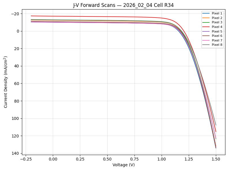
Create a SINGLE plot of the J-V curves of the forward scans with data from all pixels.
a. Remember you can copy and paste code from previous notebooks and use AI tools.
b. Also remember that you measured I-V from the pixels, so you will need to determine the current density, J, first before plotting.
# Your code hereQuestion 1: Discuss what you observe from looking at the comparison of your J-V curves. Do you have any pixels showing different behaviors?
Calculate the \(J_{sc}\) and PCE values for each pixel and save them to a CSV file. The code below will also extract the standard error (SE) of the current at key measurement points, which we will use for uncertainty propagation later in the notebook. The code will loop through this week's JV measurements and output a CSV file with the following column headers:
Pixel Number|Jsc (mA/cm^2)|SE_Jsc (mA/cm^2)|J_pmax (mA/cm^2)|V_pmax (V)|PCE|SE_Jpmax (mA/cm^2)|dV (V)|n_at_MPPNote. If you already have your own loop to do these calculations, feel free to use that. Just make sure your code also reads the
Forward_std (mA)andForward_ncolumns from the raw data so you can compute the standard error.
# Variables needed for J-V analysis
import numpy as np
import matplotlib.pyplot as plt
import pandas as pd
import os

# ===== ANSWER KEY: Process Week 7 (current week) =====
# Update these variables for the current week's data
date_str = "2026_02_04"
cell_id  = "R34"
area_cm2 = 0.14
P_in = 99.8
pixels = range(1, 9)

# Path to the data files (adjust if using Colab or different directory)
data_dir = "sample-data/Week 1/"  # for current week (2026-02-04)

# Column names matching the CSV output from measurement software
COL_V          = "Voltage (V)"
COL_Forward_mA = "Forward_mean (mA)"
COL_Fwd_std    = "Forward_std (mA)"
COL_Fwd_n      = "Forward_n"

# Store raw DataFrames and JV DataFrames for each pixel
raw_data = {}
jv_data  = {}

# Load each pixel's data
for n in pixels:
    fname = os.path.join(data_dir, f"{date_str}_IV_cell{cell_id}_pixel{n}.csv")
    try:
        df_raw = pd.read_csv(fname)
        raw_data[n] = df_raw

        df_jv = pd.DataFrame({
            "Voltage (V)": df_raw[COL_V].astype(float),
            "Current Density (mA/cm^2)": df_raw[COL_Forward_mA].astype(float) / area_cm2
        }).sort_values("Voltage (V)").reset_index(drop=True)

        df_jv["Power Density (mW/cm^2)"] = (
            df_jv["Voltage (V)"] * df_jv["Current Density (mA/cm^2)"]
        )

        jv_data[n] = df_jv
        print(f"[ok] Loaded pixel {n}")

    except FileNotFoundError:
        print(f"[skip] Pixel {n}: file not found ({fname})")
    except Exception as e:
        print(f"[skip] Pixel {n}: error reading {fname}: {e}")

# --- Plot all J-V curves on a single plot ---
fig, ax = plt.subplots(figsize=(8, 6))
for n in sorted(jv_data.keys()):
    jv = jv_data[n]
    ax.plot(jv["Voltage (V)"], jv["Current Density (mA/cm^2)"], label=f"Pixel {n}")
ax.set_xlabel("Voltage (V)")
ax.set_ylabel("Current Density (mA/cm$^2$)")
ax.set_title(f"J-V Forward Scans — {date_str} Cell {cell_id}")
ax.legend(fontsize=8)
ax.grid(True, alpha=0.4)
ax.invert_yaxis()
plt.tight_layout()
plt.show()

# --- Calculate PCE parameters and SE-based uncertainties ---
rows = []
valid_pixels = sorted(jv_data.keys())

for n in valid_pixels:
    jv  = jv_data[n]
    raw = raw_data[n].sort_values(COL_V).reset_index(drop=True)

    V = jv["Voltage (V)"].to_numpy()
    J = jv["Current Density (mA/cm^2)"].to_numpy()

    # Standard PV parameters
    Voc = float(np.interp(0.0, J, V))
    Jsc = float(np.interp(0.0, V, J))
    P   = V * J
    idx_pmax = int(np.argmin(P))
    Vmp = float(V[idx_pmax])
    Jmp = float(J[idx_pmax])

    denom = abs(Jsc) * Voc
    FF  = (Vmp * abs(Jmp)) / denom if denom != 0 else np.nan
    PCE = ((Voc * abs(Jsc) * FF) / P_in) * 100 if P_in != 0 else np.nan

    # Standard Error at the MPP
    std_mA_mpp = float(raw[COL_Fwd_std].iloc[idx_pmax])
    n_mpp      = float(raw[COL_Fwd_n].iloc[idx_pmax])

    if n_mpp > 1:
        SE_I_mpp = std_mA_mpp / np.sqrt(n_mpp)
        SE_J_mpp = SE_I_mpp / area_cm2
    else:
        SE_J_mpp = np.nan
        print(f"  [warn] Pixel {n}: n=1 at MPP, SE undefined")

    # Standard Error at V=0 (for Jsc uncertainty)
    idx_v0 = int(np.argmin(np.abs(raw[COL_V].to_numpy())))
    std_mA_v0 = float(raw[COL_Fwd_std].iloc[idx_v0])
    n_v0      = float(raw[COL_Fwd_n].iloc[idx_v0])

    if n_v0 > 1:
        SE_Jsc = (std_mA_v0 / np.sqrt(n_v0)) / area_cm2
    else:
        SE_Jsc = np.nan

    # Voltage uncertainty: half the voltage step size
    if len(V) > 1:
        voltage_step = float(np.median(np.abs(np.diff(V))))
        dV = voltage_step / 2.0
    else:
        dV = np.nan

    rows.append({
        "Pixel Number":        n,
        "Jsc (mA/cm^2)":      Jsc,
        "SE_Jsc (mA/cm^2)":   SE_Jsc,
        "J_pmax (mA/cm^2)":   Jmp,
        "V_pmax (V)":         Vmp,
        "PCE":                PCE,
        "SE_Jpmax (mA/cm^2)": SE_J_mpp,
        "dV (V)":             dV,
        "n_at_MPP":           n_mpp,
    })

out_name = f"{date_str}_jsc_pce_cell{cell_id}.csv"
df_out = pd.DataFrame(rows)

if df_out.empty:
    print("[warn] No valid pixels found.")
else:
    df_out.sort_values("Pixel Number").to_csv(out_name, index=False)
    print(f"\n[ok] Wrote {out_name}")
    display(df_out)
[ok] Loaded pixel 1
[ok] Loaded pixel 2
[ok] Loaded pixel 3
[ok] Loaded pixel 4
[ok] Loaded pixel 5
[ok] Loaded pixel 6
[ok] Loaded pixel 7
[ok] Loaded pixel 8
[ok] Wrote 2026_02_04_jsc_pce_cellR34.csv
| Pixel Number | Jsc (mA/cm^2) | SE_Jsc (mA/cm^2) | J_pmax (mA/cm^2) | V_pmax (V) | PCE | SE_Jpmax (mA/cm^2) | dV (V) | n_at_MPP | |
|---|---|---|---|---|---|---|---|---|---|
| 0 | 1 | -10.125429 | 0.001705 | -8.239857 | 1.00 | 8.256370 | 0.003939 | 0.01 | 10.0 |
| 1 | 2 | -12.444500 | 0.003228 | -10.308714 | 1.00 | 10.329373 | 0.004064 | 0.01 | 10.0 |
| 2 | 3 | -12.956500 | 0.005053 | -10.836143 | 1.00 | 10.857859 | 0.005148 | 0.01 | 10.0 |
| 3 | 4 | -17.124143 | 0.002690 | -14.687643 | 1.02 | 15.011419 | 0.003901 | 0.01 | 10.0 |
| 4 | 5 | -10.037500 | 0.002731 | -8.250357 | 1.00 | 8.266891 | 0.004242 | 0.01 | 10.0 |
| 5 | 6 | -10.926071 | 0.004064 | -8.839214 | 1.00 | 8.856928 | 0.004710 | 0.01 | 10.0 |
| 6 | 7 | -10.257786 | 0.004213 | -8.279286 | 0.98 | 8.129960 | 0.006024 | 0.01 | 10.0 |
| 7 | 8 | -12.781143 | 0.003632 | -10.585357 | 1.00 | 10.606570 | 0.006709 | 0.01 | 10.0 |
NOTE. Even though your code gives you confirmation that it has successfully written your CSV, always open the file and check to make sure the data you meant to write is actually there.
1.1 Measurement Uncertainty and Error Bars
Last week in lecture, we discussed error propagation and the importance of measurement uncertainty in the context of asking and answering scientific questions. To this end, we will calculate uncertainties in our JV measurements, propagate those uncertainties through our analysis, and then include error bars in our plots.
1.1.1 Standard Error of the Mean
When we take repeated measurements of the same quantity, we expect some variability from one measurement to the next. Two important statistical quantities help us characterize this variability:
Standard Deviation (std) tells us how spread out individual measurements are. If you measured a current 10 times, the standard deviation describes the typical spread of those 10 values.
Standard Error of the Mean (SE) tells us how precisely we know the average of those measurements:
\[SE = \frac{\text{std}}{\sqrt{n}}\]
where \(n\) is the number of repeated measurements. As we take more measurements, the standard error gets smaller — our estimate of the mean becomes more precise.
Why SE instead of std? When we report \(J_{pmax}\), \(J_{sc}\), or any other parameter, we are using the mean value from our repeated measurements. The appropriate uncertainty for a mean value is the standard error, not the standard deviation.
Our measurement software already computes the mean, standard deviation, and \(n\) for each voltage point. The columns Forward_std (mA) and Forward_n in your J-V data files contain exactly what we need:
\[SE_{J} = \frac{\texttt{Forward\_std (mA)}}{\sqrt{\texttt{Forward\_n}}} \div \texttt{pixel area}\]
The code above already extracted these SE values at the maximum power point and at \(V = 0\).
1.1.2 Uncertainty Propagation for PCE
We will propagate the uncertainty using the following formula:
\[\delta f = \sqrt{\left(\frac{\partial f}{\partial x}\right)^{2}(\delta x)^{2} + \left(\frac{\partial f}{\partial y}\right)^{2}(\delta y)^{2} + \left(\frac{\partial f}{\partial z}\right)^{2}(\delta z)^{2}}\]
Recall that:
\[PCE = \frac{|J_{pmax}| \times V_{pmax}}{P_{in}} \times 100\%\]
so the uncertainty in the PCE is:
\[\delta_{PCE} = PCE \times \sqrt{\left(\frac{\delta J_{pmax}}{J_{pmax}}\right)^2 + \left(\frac{\delta V_{pmax}}{V_{pmax}}\right)^2 + \left(\frac{\delta P_{in}}{P_{in}}\right)^2}\]
where:
- \(\delta J_{pmax}\) = standard error of the current density at the maximum power point (from our data)
- \(\delta V_{pmax}\) = half the voltage step size (instrument resolution)
- \(\delta P_{in}\) = \(0.9 mW/cm^{2}\) (calibration uncertainty of the solar simulator)
The code in the next cell computes this propagation automatically using the SE values extracted above.
1.1.3 Which uncertainty matters most?
Notice that we have three very different types of uncertainty entering the propagation:
| Source | Type | What it represents |
|---|---|---|
| \(\delta J_{pmax}\) | Statistical (SE from repeated measurements) | How precisely we know the mean current at the MPP |
| \(\delta V_{pmax}\) | Instrumental (voltage step resolution) | The finite spacing between voltage set-points |
| \(\delta P_{in}\) | Calibration (solar simulator spec) | How well we know the incident light power |
After running the code below, look at the relative uncertainty breakdown it prints. Which of these three terms dominates the total PCE uncertainty? What does that tell you about what limits the precision of your measurement — and what you would need to change to reduce it?
# --- PCE Uncertainty Propagation using Standard Error (Week 7) ---
df = pd.read_csv(f"{date_str}_jsc_pce_cell{cell_id}.csv")

# Time variable — this is Week 7 (168 hours after baseline)
t = 168
df["Time (hr)"] = t

# Uncertainty in light power (from solar simulator calibration)
dP_in = 0.9  # mW/cm^2

# --- Propagate uncertainty for PCE ---
J_abs   = np.abs(df["J_pmax (mA/cm^2)"].to_numpy())
V_vals  = np.abs(df["V_pmax (V)"].to_numpy())
PCE_vals = df["PCE"].to_numpy()
dJ      = df["SE_Jpmax (mA/cm^2)"].to_numpy()
dV      = df["dV (V)"].to_numpy()

# Relative uncertainties
rel_J   = dJ / J_abs
rel_V   = dV / V_vals
rel_Pin = dP_in / P_in

# PCE uncertainty (in percentage points, same units as PCE)
df["PCE_uncertainty (%)"] = PCE_vals * np.sqrt(rel_J**2 + rel_V**2 + rel_Pin**2)

# Jsc uncertainty for reporting
df["Jsc_uncertainty (mA/cm^2)"] = df["SE_Jsc (mA/cm^2)"]

# Write final output
out_name = f"{date_str}_jsc_pce_uncertainties_cell{cell_id}.csv"
cols_to_write = [
    "Pixel Number", "Time (hr)",
    "Jsc (mA/cm^2)", "Jsc_uncertainty (mA/cm^2)",
    "PCE", "PCE_uncertainty (%)"
]
df[cols_to_write].to_csv(out_name, index=False)
print(f"[ok] Wrote {out_name}")
display(df[cols_to_write])

# Print a summary for quick review
print("\n--- Summary ---")
for _, row in df.iterrows():
    pix = int(row["Pixel Number"])
    pce = row["PCE"]
    dpce = row["PCE_uncertainty (%)"]
    jsc = row["Jsc (mA/cm^2)"]
    djsc = row["Jsc_uncertainty (mA/cm^2)"]
    print(f"  Pixel {pix}: PCE = {pce:.2f} +/- {dpce:.2f} %,  "
          f"Jsc = {jsc:.3f} +/- {djsc:.3f} mA/cm^2")

# --- Relative uncertainty breakdown ---
print("\n--- Relative Uncertainty Breakdown (as %) ---")
print(f"  {'Pixel':>5s}  {'δJ/J':>8s}  {'δV/V':>8s}  {'δP/P':>8s}  {'Total':>8s}")
for _, row in df.iterrows():
    pix = int(row["Pixel Number"])
    rJ = row["SE_Jpmax (mA/cm^2)"] / abs(row["J_pmax (mA/cm^2)"]) * 100
    rV = row["dV (V)"] / abs(row["V_pmax (V)"]) * 100
    rP = dP_in / P_in * 100
    total = np.sqrt((rJ/100)**2 + (rV/100)**2 + (rP/100)**2) * 100
    print(f"  {pix:5d}  {rJ:7.3f}%  {rV:7.3f}%  {rP:7.3f}%  {total:7.3f}%")

print(f"\n  Note: δJ/J is the SE-based measurement uncertainty (statistical).")
print(f"        δV/V is the voltage step resolution (instrumental).")
print(f"        δP/P is the solar simulator calibration (systematic).")
[ok] Wrote 2026_02_04_jsc_pce_uncertainties_cellR34.csv
| Pixel Number | Time (hr) | Jsc (mA/cm^2) | Jsc_uncertainty (mA/cm^2) | PCE | PCE_uncertainty (%) | |
|---|---|---|---|---|---|---|
| 0 | 1 | 168 | -10.125429 | 0.001705 | 8.256370 | 0.111248 |
| 1 | 2 | 168 | -12.444500 | 0.003228 | 10.329373 | 0.139152 |
| 2 | 3 | 168 | -12.956500 | 0.005053 | 10.857859 | 0.146300 |
| 3 | 4 | 168 | -17.124143 | 0.002690 | 15.011419 | 0.200003 |
| 4 | 5 | 168 | -10.037500 | 0.002731 | 8.266891 | 0.111401 |
| 5 | 6 | 168 | -10.926071 | 0.004064 | 8.856928 | 0.119358 |
| 6 | 7 | 168 | -10.257786 | 0.004213 | 8.129960 | 0.110871 |
| 7 | 8 | 168 | -12.781143 | 0.003632 | 10.606570 | 0.142983 |
--- Summary ---
  Pixel 1: PCE = 8.26 +/- 0.11 %,  Jsc = -10.125 +/- 0.002 mA/cm^2
  Pixel 2: PCE = 10.33 +/- 0.14 %,  Jsc = -12.444 +/- 0.003 mA/cm^2
  Pixel 3: PCE = 10.86 +/- 0.15 %,  Jsc = -12.956 +/- 0.005 mA/cm^2
  Pixel 4: PCE = 15.01 +/- 0.20 %,  Jsc = -17.124 +/- 0.003 mA/cm^2
  Pixel 5: PCE = 8.27 +/- 0.11 %,  Jsc = -10.037 +/- 0.003 mA/cm^2
  Pixel 6: PCE = 8.86 +/- 0.12 %,  Jsc = -10.926 +/- 0.004 mA/cm^2
  Pixel 7: PCE = 8.13 +/- 0.11 %,  Jsc = -10.258 +/- 0.004 mA/cm^2
  Pixel 8: PCE = 10.61 +/- 0.14 %,  Jsc = -12.781 +/- 0.004 mA/cm^2

--- Relative Uncertainty Breakdown (as %) ---
  Pixel      δJ/J      δV/V      δP/P     Total
      1    0.048%    1.000%    0.902%    1.347%
      2    0.039%    1.000%    0.902%    1.347%
      3    0.048%    1.000%    0.902%    1.347%
      4    0.027%    0.980%    0.902%    1.332%
      5    0.051%    1.000%    0.902%    1.348%
      6    0.053%    1.000%    0.902%    1.348%
      7    0.073%    1.020%    0.902%    1.364%
      8    0.063%    1.000%    0.902%    1.348%

  Note: δJ/J is the SE-based measurement uncertainty (statistical).
        δV/V is the voltage step resolution (instrumental).
        δP/P is the solar simulator calibration (systematic).
1.1.4 Interpreting the Uncertainty Breakdown
Look at the relative uncertainty table printed above. You should notice that:
- \(\delta J / J\) is very small (typically < 0.1%). With \(n\) repeated measurements at each voltage, the standard error of the mean current is tiny — our instrument measures current very precisely and reproducibly.
- \(\delta V / V\) and \(\delta P_{in} / P_{in}\) dominate (each ~1%). These are not statistical uncertainties from repeated measurements — they are fixed properties of the instrument (the voltage step size chosen for the sweep) and the calibration of the solar simulator.
This reveals something important about this experiment: the precision of the PCE measurement is limited by instrument resolution and calibration, not by measurement repeatability. Taking more current measurements (increasing \(n\)) would make \(\delta J / J\) even smaller, but would barely change the total uncertainty because the other two terms dominate.
Question 2: Looking at the breakdown, which term contributes the most to the total PCE uncertainty? If you wanted to cut the PCE uncertainty in half, what would you need to change about the measurement — and what would not help?
Sample Answer: The voltage step resolution (\(\delta V / V \approx 1\%\)) is the largest single contributor, followed closely by the solar simulator calibration (\(\delta P_{in} / P_{in} \approx 0.9\%\)). Together these two instrumental/calibration terms account for nearly all of the total uncertainty (~1.3%). The statistical measurement uncertainty (\(\delta J / J < 0.1\%\)) is negligible by comparison. To reduce the PCE uncertainty, you would need to: (1) use finer voltage steps in the J-V sweep (e.g., 0.01 V instead of 0.02 V), and/or (2) improve the solar simulator calibration. Simply taking more repeated sweeps (increasing \(n\)) would not meaningfully help, because it only reduces the already-tiny \(\delta J / J\) term.
Repeat the J-V analysis above for your other weeks of data. For each week, upload the raw JV CSV files from your team's shared Google Drive folder, update
date_strandt, and re-run the code to generate the uncertainty CSV files. (The originals will remain in Google Drive — uploading just creates a working copy in Colab.)Once you have uncertainty CSV files for all of your weeks, you are ready to plot.
Below we process the **Baseline** measurements (2026-01-28, t = 0 hr) using the same approach.
# ===== ANSWER KEY: Process Baseline (Week 6, t = 0 hr) =====
date_str_bl = "2026_01_28"
t_bl = 0
data_dir_bl = "sample-data/Baseline Measurements/"

raw_data_bl = {}
jv_data_bl  = {}

for n in pixels:
    fname = os.path.join(data_dir_bl, f"{date_str_bl}_IV_cell{cell_id}_pixel{n}.csv")
    try:
        df_raw = pd.read_csv(fname)
        raw_data_bl[n] = df_raw

        df_jv = pd.DataFrame({
            "Voltage (V)": df_raw[COL_V].astype(float),
            "Current Density (mA/cm^2)": df_raw[COL_Forward_mA].astype(float) / area_cm2
        }).sort_values("Voltage (V)").reset_index(drop=True)

        df_jv["Power Density (mW/cm^2)"] = (
            df_jv["Voltage (V)"] * df_jv["Current Density (mA/cm^2)"]
        )
        jv_data_bl[n] = df_jv
        print(f"[ok] Loaded baseline pixel {n}")
    except FileNotFoundError:
        print(f"[skip] Pixel {n}: file not found ({fname})")

# Calculate PCE + SE for baseline
rows_bl = []
for n in sorted(jv_data_bl.keys()):
    jv  = jv_data_bl[n]
    raw = raw_data_bl[n].sort_values(COL_V).reset_index(drop=True)
    V = jv["Voltage (V)"].to_numpy()
    J = jv["Current Density (mA/cm^2)"].to_numpy()

    Voc = float(np.interp(0.0, J, V))
    Jsc = float(np.interp(0.0, V, J))
    P   = V * J
    idx_pmax = int(np.argmin(P))
    Vmp = float(V[idx_pmax])
    Jmp = float(J[idx_pmax])
    denom = abs(Jsc) * Voc
    FF  = (Vmp * abs(Jmp)) / denom if denom != 0 else np.nan
    PCE = ((Voc * abs(Jsc) * FF) / P_in) * 100 if P_in != 0 else np.nan

    std_mA_mpp = float(raw[COL_Fwd_std].iloc[idx_pmax])
    n_mpp = float(raw[COL_Fwd_n].iloc[idx_pmax])
    SE_J_mpp = (std_mA_mpp / np.sqrt(n_mpp)) / area_cm2 if n_mpp > 1 else np.nan

    idx_v0 = int(np.argmin(np.abs(raw[COL_V].to_numpy())))
    SE_Jsc = (float(raw[COL_Fwd_std].iloc[idx_v0]) / np.sqrt(float(raw[COL_Fwd_n].iloc[idx_v0]))) / area_cm2

    voltage_step = float(np.median(np.abs(np.diff(V))))
    dV_bl = voltage_step / 2.0

    rows_bl.append({
        "Pixel Number": n, "Jsc (mA/cm^2)": Jsc, "SE_Jsc (mA/cm^2)": SE_Jsc,
        "J_pmax (mA/cm^2)": Jmp, "V_pmax (V)": Vmp, "PCE": PCE,
        "SE_Jpmax (mA/cm^2)": SE_J_mpp, "dV (V)": dV_bl, "n_at_MPP": n_mpp,
    })

df_bl = pd.DataFrame(rows_bl)
df_bl.sort_values("Pixel Number").to_csv(f"{date_str_bl}_jsc_pce_cell{cell_id}.csv", index=False)
print(f"\n[ok] Wrote {date_str_bl}_jsc_pce_cell{cell_id}.csv")

# Propagate uncertainty for baseline
df_bl = pd.read_csv(f"{date_str_bl}_jsc_pce_cell{cell_id}.csv")
df_bl["Time (hr)"] = t_bl

J_abs_bl   = np.abs(df_bl["J_pmax (mA/cm^2)"].to_numpy())
V_vals_bl  = np.abs(df_bl["V_pmax (V)"].to_numpy())
PCE_vals_bl = df_bl["PCE"].to_numpy()
dJ_bl      = df_bl["SE_Jpmax (mA/cm^2)"].to_numpy()
dV_bl2     = df_bl["dV (V)"].to_numpy()

rel_J_bl   = dJ_bl / J_abs_bl
rel_V_bl   = dV_bl2 / V_vals_bl
rel_Pin_bl = dP_in / P_in

df_bl["PCE_uncertainty (%)"] = PCE_vals_bl * np.sqrt(rel_J_bl**2 + rel_V_bl**2 + rel_Pin_bl**2)
df_bl["Jsc_uncertainty (mA/cm^2)"] = df_bl["SE_Jsc (mA/cm^2)"]

cols_to_write = ["Pixel Number", "Time (hr)", "Jsc (mA/cm^2)", "Jsc_uncertainty (mA/cm^2)", "PCE", "PCE_uncertainty (%)"]
df_bl[cols_to_write].to_csv(f"{date_str_bl}_jsc_pce_uncertainties_cell{cell_id}.csv", index=False)
print(f"[ok] Wrote {date_str_bl}_jsc_pce_uncertainties_cell{cell_id}.csv")
display(df_bl[cols_to_write])
[ok] Loaded baseline pixel 1
[ok] Loaded baseline pixel 2
[ok] Loaded baseline pixel 3
[ok] Loaded baseline pixel 4
[ok] Loaded baseline pixel 5
[ok] Loaded baseline pixel 6
[ok] Loaded baseline pixel 7
[ok] Loaded baseline pixel 8
[ok] Wrote 2026_01_28_jsc_pce_cellR34.csv
[ok] Wrote 2026_01_28_jsc_pce_uncertainties_cellR34.csv
| Pixel Number | Time (hr) | Jsc (mA/cm^2) | Jsc_uncertainty (mA/cm^2) | PCE | PCE_uncertainty (%) | |
|---|---|---|---|---|---|---|
| 0 | 1 | 0 | -9.827143 | 0.003395 | 8.205501 | 0.111795 |
| 1 | 2 | 0 | -11.968929 | 0.003811 | 10.264243 | 0.138368 |
| 2 | 3 | 0 | -12.745571 | 0.003971 | 11.094976 | 0.149457 |
| 3 | 4 | 0 | -16.440714 | 0.003756 | 14.763527 | 0.198888 |
| 4 | 5 | 0 | -9.153857 | 0.002785 | 7.635541 | 0.104089 |
| 5 | 6 | 0 | -10.080857 | 0.003738 | 8.402949 | 0.113341 |
| 6 | 7 | 0 | -9.587857 | 0.004109 | 7.777295 | 0.105989 |
| 7 | 8 | 0 | -11.352500 | 0.002959 | 9.525981 | 0.128376 |
# ===== ANSWER KEY: Multi-week PCE plot with correct file names =====
files = [
    "2026_01_28_jsc_pce_uncertainties_cellR34.csv",  # Baseline (t=0)
    "2026_02_04_jsc_pce_uncertainties_cellR34.csv",  # Week 1 (t=168)
]

dfs = []
for f in files:
    try:
        d = pd.read_csv(f)
        d["source_file"] = f
        dfs.append(d)
    except FileNotFoundError:
        print(f"[skip] missing file: {f}")

if not dfs:
    raise SystemExit("No data files loaded. Check file names above.")

all_df = pd.concat(dfs, ignore_index=True)

need = ["Pixel Number", "Time (hr)", "PCE", "PCE_uncertainty (%)"]
missing = [c for c in need if c not in all_df.columns]
if missing:
    raise ValueError(f"Missing required columns in data: {missing}")

all_df["Pixel Number"] = pd.to_numeric(all_df["Pixel Number"], errors="coerce").astype("Int64")
all_df["Time (hr)"]    = pd.to_numeric(all_df["Time (hr)"], errors="coerce")
all_df["PCE"]          = pd.to_numeric(all_df["PCE"], errors="coerce")
all_df["PCE_uncertainty (%)"] = pd.to_numeric(all_df["PCE_uncertainty (%)"], errors="coerce")

all_df = (
    all_df.dropna(subset=["Pixel Number", "Time (hr)", "PCE"])
          .drop_duplicates(subset=["Pixel Number", "Time (hr)"], keep="last")
)

pixels_present = sorted(all_df["Pixel Number"].dropna().unique().astype(int))

fig, ax = plt.subplots(figsize=(9, 6))
markers = ["o", "s", "^", "D", "v", ">", "x", "*"]

for i, pix in enumerate(pixels_present):
    d = all_df[all_df["Pixel Number"] == pix].sort_values("Time (hr)")
    if d.empty:
        continue
    marker = markers[i % len(markers)]
    ax.errorbar(
        d["Time (hr)"].to_numpy(),
        d["PCE"].to_numpy(),
        yerr=d["PCE_uncertainty (%)"].to_numpy(),
        fmt=marker, capsize=4, label=f"Pixel {pix}"
    )

ax.set_xlabel("Time (hr)")
ax.set_ylabel("PCE (%)")
ax.set_title(f"PCE vs Time - Cell {cell_id}")
ax.grid(True, alpha=0.4)
ax.legend(fontsize=8, title="Pixels", ncols=2)
plt.tight_layout()
plt.show()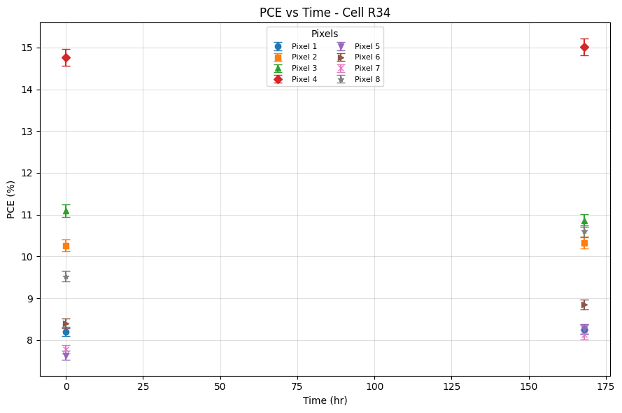
Congratulations! That was a bunch of new code, but you will have to make minimal edits to use it in upcoming weeks.
Question 3: Discuss what you observe from looking at the PCE over time. Has anything changed over the past few weeks?
1.2 EQE Analysis with Uncertainty
The External Quantum Efficiency at each wavelength is:
\[EQE(\lambda) = \frac{I(\lambda)}{P(\lambda)} \times \frac{hc}{e\lambda}\]
where \(I(\lambda)\) is the measured photocurrent and \(P(\lambda)\) is the incident optical power at wavelength \(\lambda\).
Since EQE is a ratio of two measured quantities (each with their own uncertainty), we can propagate the uncertainties using the same approach as for PCE:
\[\frac{\delta EQE}{EQE} = \sqrt{\left(\frac{\delta I}{I}\right)^2 + \left(\frac{\delta P}{P}\right)^2}\]
where:
- \(\delta I = SE_I = \frac{\texttt{Current\_std (nA)}}{\sqrt{n_I}}\)
- \(\delta P = SE_P = \frac{\texttt{Power\_std (uW)}}{\sqrt{n_P}}\)
This gives us an uncertainty band around each EQE curve, allowing us to assess whether changes in EQE between weeks are statistically significant.
As a reminder, the EQE data files have the following columns:
- Power data:
Wavelength (nm),Power_mean (uW),Power_std (uW),n - Current data:
Wavelength (nm),Current_mean (nA),Current_std (nA),n
- The code below calculates EQE and its uncertainty for each pixel and saves the results to a CSV file.
- The plotting cells that follow create EQE curves with shaded uncertainty bands.
# --- EQE Calculation with Standard Error Uncertainty (Week 7) ---

# Physical constants
h = 6.62607015e-34       # Planck's constant (J*s)
c = 3.0e8                # Speed of light (m/s)
e_charge = 1.602176634e-19  # Elementary charge (C)

# ===== ANSWER KEY: Use data_dir for correct file paths =====
power_fname = os.path.join(data_dir, f"{date_str}_power_cell{cell_id}.csv")
try:
    power_data = pd.read_csv(power_fname)
    print(f"[ok] Loaded power data: {power_fname}")
except FileNotFoundError:
    print(f"[error] Power file not found: {power_fname}")

wavelength_nm = power_data["Wavelength (nm)"].to_numpy()
wavelength_m  = wavelength_nm * 1e-9

P_mean_uW = power_data["Power_mean (uW)"].to_numpy()
P_std_uW  = power_data["Power_std (uW)"].to_numpy()
n_P       = power_data["n"].to_numpy().astype(float)
SE_P_uW = np.where(n_P > 1, P_std_uW / np.sqrt(n_P), np.nan)

eqe_df = pd.DataFrame({"Wavelength (nm)": wavelength_nm})

for pix in pixels:
    curr_fname = os.path.join(data_dir, f"{date_str}_current_cell{cell_id}_pixel{pix}.csv")
    try:
        curr_data = pd.read_csv(curr_fname)
        I_mean_nA = curr_data["Current_mean (nA)"].to_numpy()
        I_std_nA  = curr_data["Current_std (nA)"].to_numpy()
        n_I       = curr_data["n"].to_numpy().astype(float)
        SE_I_nA = np.where(n_I > 1, I_std_nA / np.sqrt(n_I), np.nan)

        I_mean_A = I_mean_nA * 1e-9
        SE_I_A   = SE_I_nA * 1e-9
        P_mean_W = P_mean_uW * 1e-6
        SE_P_W   = SE_P_uW * 1e-6

        eqe_vals = (I_mean_A / P_mean_W) * (h * c) / (e_charge * wavelength_m)
        rel_I = SE_I_A / np.abs(I_mean_A)
        rel_P = SE_P_W / np.abs(P_mean_W)
        eqe_unc = np.abs(eqe_vals) * np.sqrt(rel_I**2 + rel_P**2)

        eqe_df[f"eqe_pix{pix}"]     = eqe_vals
        eqe_df[f"eqe_unc_pix{pix}"] = eqe_unc
        print(f"[ok] Pixel {pix}: peak EQE = {np.nanmax(eqe_vals):.4f} ({np.nanmax(eqe_vals)*100:.1f}%)")
    except FileNotFoundError:
        print(f"[skip] Pixel {pix}: current file not found ({curr_fname})")

eqe_out = f"{date_str}_eqe_cell{cell_id}.csv"
eqe_df.to_csv(eqe_out, index=False)
print(f"\n[ok] Wrote {eqe_out}")

# ===== Also process baseline EQE =====
power_fname_bl = os.path.join(data_dir_bl, f"{date_str_bl}_power_cell{cell_id}.csv")
power_data_bl = pd.read_csv(power_fname_bl)
P_mean_uW_bl = power_data_bl["Power_mean (uW)"].to_numpy()
P_std_uW_bl  = power_data_bl["Power_std (uW)"].to_numpy()
n_P_bl       = power_data_bl["n"].to_numpy().astype(float)
SE_P_uW_bl   = np.where(n_P_bl > 1, P_std_uW_bl / np.sqrt(n_P_bl), np.nan)

eqe_df_bl = pd.DataFrame({"Wavelength (nm)": power_data_bl["Wavelength (nm)"].to_numpy()})
wavelength_m_bl = power_data_bl["Wavelength (nm)"].to_numpy() * 1e-9

for pix in sorted(jv_data_bl.keys()):
    curr_fname_bl = os.path.join(data_dir_bl, f"{date_str_bl}_current_cell{cell_id}_pixel{pix}.csv")
    try:
        curr_data_bl = pd.read_csv(curr_fname_bl)
        I_nA = curr_data_bl["Current_mean (nA)"].to_numpy()
        I_std = curr_data_bl["Current_std (nA)"].to_numpy()
        n_I = curr_data_bl["n"].to_numpy().astype(float)
        SE_I = np.where(n_I > 1, I_std / np.sqrt(n_I), np.nan)

        I_A = I_nA * 1e-9; SE_I_A2 = SE_I * 1e-9
        P_W = P_mean_uW_bl * 1e-6; SE_P_W2 = SE_P_uW_bl * 1e-6

        eqe_v = (I_A / P_W) * (h * c) / (e_charge * wavelength_m_bl)
        eqe_u = np.abs(eqe_v) * np.sqrt((SE_I_A2/np.abs(I_A))**2 + (SE_P_W2/np.abs(P_W))**2)

        eqe_df_bl[f"eqe_pix{pix}"]     = eqe_v
        eqe_df_bl[f"eqe_unc_pix{pix}"] = eqe_u
        print(f"[ok] Baseline pixel {pix}: peak EQE = {np.nanmax(eqe_v):.4f}")
    except FileNotFoundError:
        print(f"[skip] Baseline pixel {pix}: not found")

eqe_out_bl = f"{date_str_bl}_eqe_cell{cell_id}.csv"
eqe_df_bl.to_csv(eqe_out_bl, index=False)
print(f"[ok] Wrote {eqe_out_bl}")
[ok] Loaded power data: sample-data/Week 1/2026_02_04_power_cellR34.csv
[ok] Pixel 1: peak EQE = 0.9588 (95.9%)
[ok] Pixel 2: peak EQE = 0.9334 (93.3%)
[ok] Pixel 3: peak EQE = 0.9252 (92.5%)
[ok] Pixel 4: peak EQE = 0.8964 (89.6%)
[ok] Pixel 5: peak EQE = 0.9278 (92.8%)
[ok] Pixel 6: peak EQE = 0.9117 (91.2%)
[ok] Pixel 7: peak EQE = 0.9419 (94.2%)
[ok] Pixel 8: peak EQE = 0.9323 (93.2%)
[ok] Wrote 2026_02_04_eqe_cellR34.csv
[ok] Baseline pixel 1: peak EQE = 0.9792
[ok] Baseline pixel 2: peak EQE = 0.9707
[ok] Baseline pixel 3: peak EQE = 0.9605
[ok] Baseline pixel 4: peak EQE = 0.9531
[ok] Baseline pixel 5: peak EQE = 0.9770
[ok] Baseline pixel 6: peak EQE = 0.9720
[ok] Baseline pixel 7: peak EQE = 0.9686
[ok] Baseline pixel 8: peak EQE = 0.9748
[ok] Wrote 2026_01_28_eqe_cellR34.csv
# --- EQE Plots with Shaded Uncertainty Bands (This Week) ---
eqe_df_plot = pd.read_csv(f"{date_str}_eqe_cell{cell_id}.csv")
wl = eqe_df_plot["Wavelength (nm)"].to_numpy()

fig, axes = plt.subplots(4, 2, figsize=(12, 16))
axes_flat = axes.flatten()

for i in range(8):
    ax = axes_flat[i]
    pix = i + 1
    col_eqe = f"eqe_pix{pix}"
    col_unc = f"eqe_unc_pix{pix}"

    if col_eqe not in eqe_df_plot.columns:
        ax.set_visible(False)
        continue

    eqe_vals = eqe_df_plot[col_eqe].to_numpy()
    ax.plot(wl, eqe_vals, 'b-', label="EQE")

    if col_unc in eqe_df_plot.columns:
        eqe_unc = eqe_df_plot[col_unc].to_numpy()
        ax.fill_between(wl,
                        eqe_vals - eqe_unc,
                        eqe_vals + eqe_unc,
                        alpha=0.3, color='blue',
                        label="SE uncertainty")

    ax.set_title(f"Pixel {pix}")
    ax.set_xlabel("Wavelength (nm)")
    ax.set_ylabel("EQE")
    ax.legend(fontsize=8)
    ax.set_ylim(bottom=0)

plt.suptitle(f"EQE with Uncertainty — {date_str} Cell {cell_id}", fontsize=14)
plt.tight_layout()
plt.show()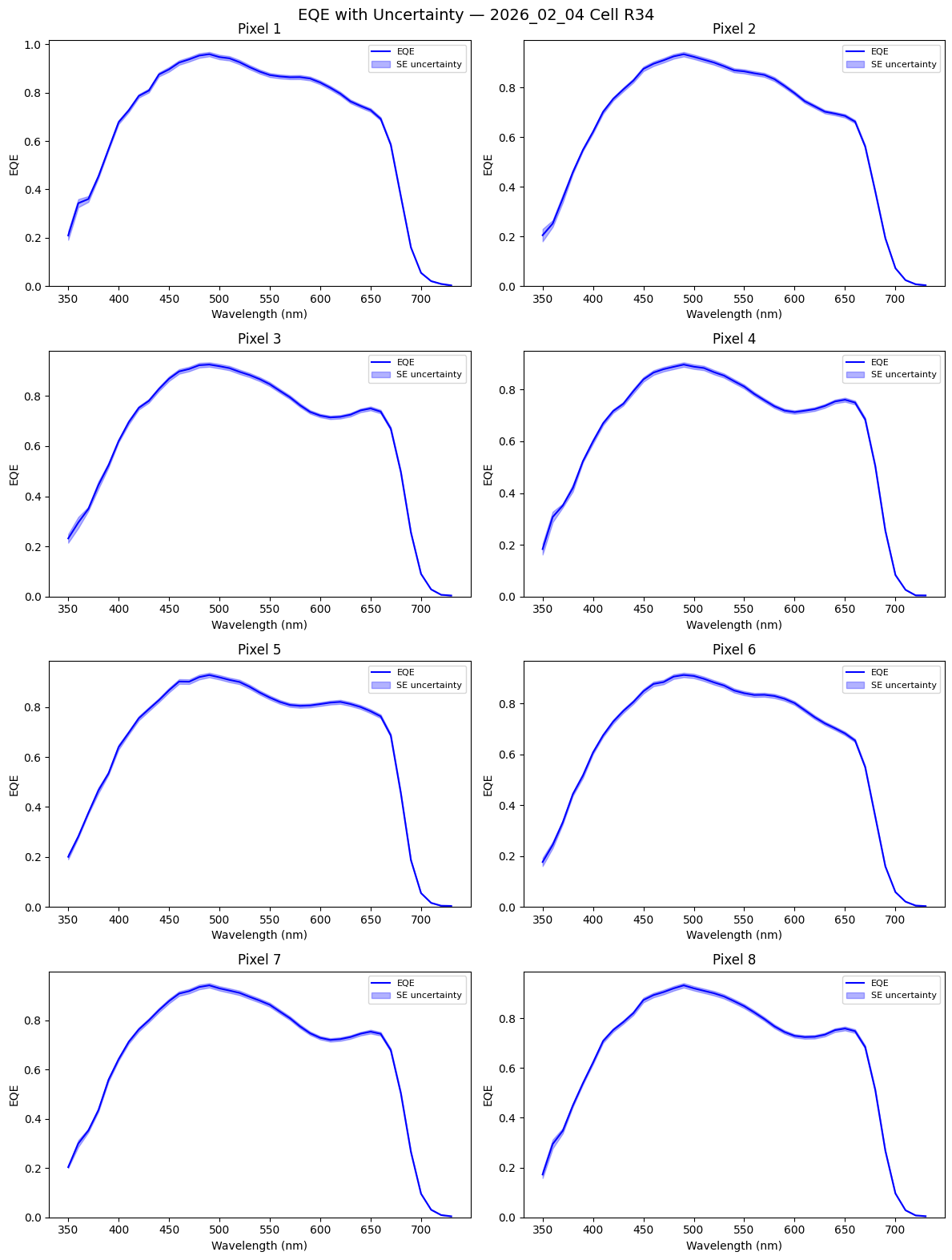
# ===== ANSWER KEY: Multi-Week EQE Comparison with correct file names =====
eqe_files = {
    "Baseline (0 hr)": "2026_01_28_eqe_cellR34.csv",
    "Week 1 (168 hr)": "2026_02_04_eqe_cellR34.csv",
}

colors = ['blue', 'red', 'green', 'purple', 'orange', 'brown']

eqe_weeks = {}
for label, fname in eqe_files.items():
    try:
        eqe_weeks[label] = pd.read_csv(fname)
        print(f"[ok] Loaded {label}: {fname}")
    except FileNotFoundError:
        print(f"[skip] {label}: {fname} not found")

if not eqe_weeks:
    print("[warn] No EQE files loaded.")
else:
    fig, axes = plt.subplots(4, 2, figsize=(12, 16))
    axes_flat = axes.flatten()

    for i in range(8):
        ax = axes_flat[i]
        pix = i + 1
        col_eqe = f"eqe_pix{pix}"
        col_unc = f"eqe_unc_pix{pix}"

        for j, (label, df_eqe) in enumerate(eqe_weeks.items()):
            color = colors[j % len(colors)]
            wl = df_eqe["Wavelength (nm)"].to_numpy()
            if col_eqe in df_eqe.columns:
                eqe_vals = df_eqe[col_eqe].to_numpy()
                ax.plot(wl, eqe_vals, color=color, label=label)
                if col_unc in df_eqe.columns:
                    eqe_unc = df_eqe[col_unc].to_numpy()
                    ax.fill_between(wl, eqe_vals - eqe_unc, eqe_vals + eqe_unc,
                                    alpha=0.15, color=color)

        ax.set_title(f"Pixel {pix}")
        ax.set_xlabel("Wavelength (nm)")
        ax.set_ylabel("EQE")
        ax.legend(fontsize=7)
        ax.set_ylim(bottom=0)

    plt.suptitle(f"EQE Comparison Over Time — Cell {cell_id}", fontsize=14)
    plt.tight_layout()
    plt.show()
[ok] Loaded Baseline (0 hr): 2026_01_28_eqe_cellR34.csv
[ok] Loaded Week 1 (168 hr): 2026_02_04_eqe_cellR34.csv

Question 4: Discuss what you observe from looking at the comparison of all of your EQE curves. Considering the uncertainty bands, are the changes in EQE between weeks statistically significant? At which wavelengths is the uncertainty largest relative to the EQE value, and why?
3 Use of AI (required)
- How your team used AI tools: Describe the specific tasks where AI-assisted tools were involved. For example, did AI help with writing, debugging, optimizing, or refining your code? Which components of the analysis did your team use AI on?
- When your team used AI tools: Specify at what stage(s) of your programming process you used AI. Was it during initial code development, troubleshooting, etc.?
- Which AI tools your team used: Identify the AI tools or platforms your team consulted (e.g., ChatGPT, GitHub Copilot, etc.).